Fast Radio Bursts: Review and Audio/Visual Exploration

Kyle Miller

# import stuff
	  import matplotlib.pyplot as plt
	  import numpy as np
	  import pandas as pd
	  import seaborn as sns
	  import veusz
	  from IPython.display import HTML, IFrame, Video
	  import astropy.coordinates as coord
	  import astropy.units as u
	  from astropy import constants
	  from astropy.coordinates import SkyCoord
	  import ugradio
	  import fruitbat
	  import astroquery
	  from astroquery.gaia import Gaia
	  from astropy.table import QTable

# output control
	  import warnings
	  def function_that_warns():
	      warnings.warn("deprecated", DeprecationWarning)
	  
	  with warnings.catch_warnings():
	      warnings.simplefilter("ignore")
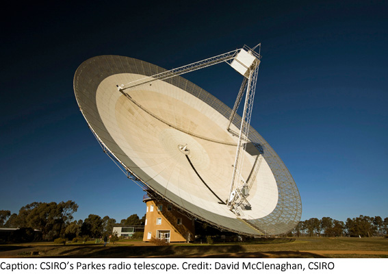
	      function_that_warns()  # this will not show a warning

Background/History

The first fast radio burst (FRB) was found in archival data from the Parkes observatory. The FRB occurred in 2001 but was noticed in 2007. It took a few more years before this mysterious new transient was recognized as a unique type of astrophysical event when more were reported.

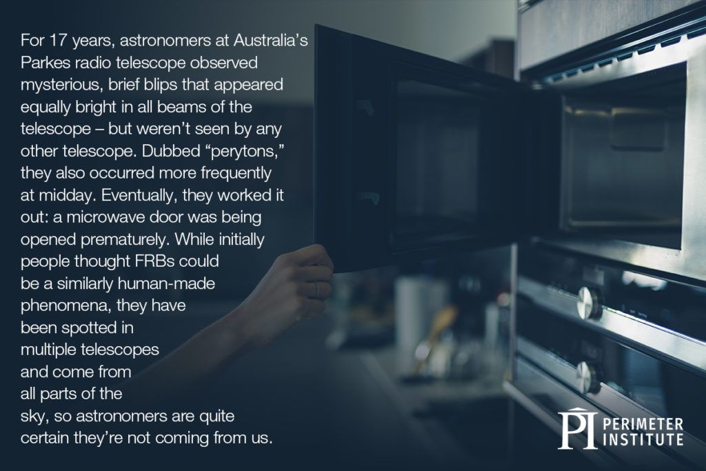
image of Parkes observatory — Parkes observatory (Austrailia) [https://www.parkes.atnf.csiro.au/]

This radio telescope was the main receiver for the Apollo 11 landing TV transmission, incidentally. Another interesting tidbit of Parkes history was the enigmatic phenomenon of “perytons”:

image of microwave oven — Perytons (mircowave EFI) [https://insidetheperimeter.ca/fast-radio-bursts-what-in-the-universe-are-they/]

Today the resolution of this radio telescope has been eclipsed by larger single dishes and interferometers. The increase in resolution is not always helpful with FRBs, however. It has been established that FRBs are generally extragalactic in origin because there is no clustering on the galactic plane. Moreover, they appear to have no identifiable pattern and so are assumed to be isotropic much like cosmology writ large. While there has only been a moderate number of FRB detections it has been estimated that about 1000 of these events happen per day across the entire sky. This would be at all values of $z$ for the redshift, which is analogous to distance modulo the metric of spacetime.

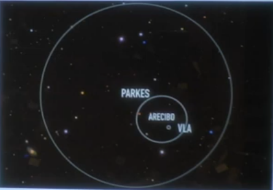
field of view of radio telescopes — Field of view (FOV) of radio telescopes [https://www.youtube.com/watch?v=PnTpOmTmedc]

This image was presented by Casey Law who has implemented a transient detection pipeline at the VLA. As the VLA is used by many scientists the computer back-end of the telescope can be simultaneously combed for transients. The program is called “realfast” and is an example of the emerging field of time domain astronomy.

What is an FRB?

Its a high energy burst in the radio band, typically found from 300 MHz to 8 GHz [Zhang2020].

online catalog of frbs: http://frbcat.org/

There is also a curated list of FRBs at: https://en.wikipedia.org/wiki/List_of_fast_radio_bursts

# read in frb data and show columns
	  frb_catalog = pd.read_csv('frbcat_csv_noindex')
	  units= ['backend', 'bandwidth [MHz]', 'beam [arcmin]', 'beam_rotation_angle [deg]',
	         'beam_semi_major_axis [arcmin]', 'beam_semi_minor_axis [arcmin]', 'bits_per_sample [bits/sample]',
	         'centre_frequency [MHz]', 'channel_bandwidth [MHz]', 'circular_poln_frac',
	         'circular_poln_frac_error', 'circular_poln_frac_frmt',
	         'circular_poln_frac_frmt_err', 'count', 'dec', 'decj',
	         'dispersion_smearing [ms]', 'dm [pc/cm^3]', 'dm_error', 'dm_frmt', 'dm_frmt_err',
	         'dm_index', 'dm_index_error', 'dm_index_frmt', 'dm_index_frmt_err',
	         'fluence', 'fluence_error_lower', 'fluence_error_upper', 'fluence_frmt',
	         'fluence_frmt_err_down', 'fluence_frmt_err_up', 'flux [Jy]',
	         'flux_error_lower', 'flux_error_upper', 'flux_frmt',
	         'flux_frmt_err_down', 'flux_frmt_err_up', 'frb_name', 'gain [K/Jy]',
	         'galactic_electron_model', 'gb [deg]', 'gl [deg]', 'linear_poln_frac',
	         'linear_poln_frac_error', 'linear_poln_frac_frmt',
	         'linear_poln_frac_frmt_err', 'mw_dm_limit', 'notes_author_x',
	         'notes_author_y', 'notes_last_modified_x', 'notes_last_modified_y',
	         'notes_note_x', 'notes_note_y', 'npol', 'o_data_link',
	         'pub_description', 'pub_link', 'pub_reference', 'pub_type', 'ra', 'raj',
	         'receiver', 'redshift_host [z]', 'redshift_inferred', 'rm', 'rm_error',
	         'sampling_time [ms]', 'scattering [ms]', 'scattering_error', 'scattering_frmt',
	         'scattering_frmt_err', 'scattering_index', 'scattering_index_error',
	         'scattering_index_frmt', 'scattering_index_frmt_err',
	         'scattering_model', 'scattering_timescale [ms]', 'snr [S/N]', 'snr_frmt',
	         'spectral_index', 'spectral_index_error', 'spectral_index_frmt',
	         'spectral_index_frmt_err', 'telescope', 'tsys [K]', 'type', 'unnamed: 0',
	         'utc', 'width [ms]', 'width_error_lower', 'width_error_upper', 'width_frmt',
	         'width_frmt_err_down', 'width_frmt_err_up']
	  frb_catalog.columns = units

# list the telescopes that have reported FRBs
	  num_telescopes = pd.unique(frb_catalog['telescope'].values).shape[0]
	  pd.unique(frb_catalog['telescope'].values)

array(['askap', 'utmost', 'srt', 'gbt', 'apertif', 'chime', 'effelsberg',
	'vla', 'dsa-10', 'fast', 'parkes', 'pushchino', 'arecibo'],
	dtype=object)

# show average stats for each telescope for FRBs
	  frb_catalog.groupby('telescope').mean()

13 rows x 79 columns

# plot flux vs. SNR
      sns.set(context="poster", style="whitegrid",
              rc={'grid.alpha':.5, 'grid.linestyle':'dotted', 'grid.color':'k',
                  "lines.linewidth":2.5, "axes.edgecolor":'k',
                  'legend.facecolor':'w', 'text.usetex':False, 'mathtext.fontset':'cm',
                  'legend.fontsize':'x-small', 'legend.framealpha':0.88,
                  'axes.formatter.use_mathtext':True, 'figure.dpi':180, 'font.family':'monospace',
                 "figure.facecolor":'none', 'axes.facecolor':'none'})
      with warnings.catch_warnings():
          warnings.simplefilter("ignore")
          sns.jointplot(data=frb_catalog, x='flux [Jy]', xlim=(-10,180), palette=sns.color_palette("hls", 13),
                        y='snr [S/N]', ylim=(-40,420), hue='telescope', space=0, height=11, ratio=7, s=155);

# plot sampling time vs. SNR
      with warnings.catch_warnings():
          warnings.simplefilter("ignore")
          sns.jointplot(data=frb_catalog, x='sampling_time [ms]', xlim=(-.5,5.5),
                        palette=sns.color_palette("hls", 13), y='snr [S/N]', ylim=(-40,420), hue='telescope',
                        space=0, height=11, ratio=7, s=155);

# plot bandwidth vs. SNR
      with warnings.catch_warnings():
          warnings.simplefilter("ignore")
          sns.jointplot(data=frb_catalog, x='bandwidth [MHz]', xlim=(-10,420),
                        palette=sns.color_palette("hls", 13),
                        y='snr [S/N]', ylim=(-40,420), hue='telescope',
                        space=0, height=11, ratio=7, s=155);

Cumulative FRBs by year

# plot histogram
      # convert the utc times to pandas_datetimes
      frb_catalog['utc'] = pd.to_datetime(frb_catalog['utc'])
      frb_catalog['utc'].sort_values()[0]
      plt.figure(figsize=(11,7), dpi=180)
      plt.axvline(x=pd.Timestamp('2001-07-24'), label="First FRB Event", alpha=.5, color='g');
      plt.axvline(x=pd.Timestamp('2007-11-01'), label="First FRB Report", alpha=.5, color='b');
      plt.axvline(x=pd.Timestamp('2013-07-05'), label="Second FRB Report", alpha=.5, color='r');
      bins = plt.hist(frb_catalog['utc'].sort_values(), cumulative=True, bins=20, histtype='stepfilled', alpha=1,
                      color='gray', zorder=2.5)
      plt.ylabel('# of FRBs reported'); plt.grid(True, linestyle='dotted', alpha=.5);
      plt.legend(loc='upper left', fontsize='x-small');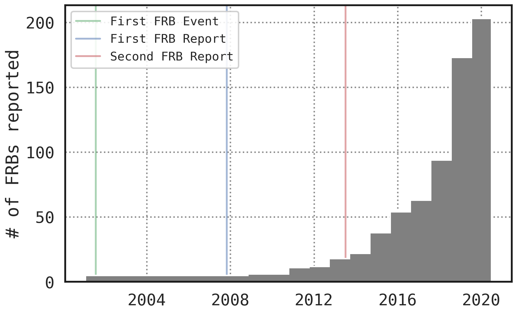

Plot sky distribution of FRBs

setup coordinates for equatorial and galactic

# get coordinates for all FRB observations
      observations = []
      for i,obs_name in enumerate(frb_catalog['frb_name']):
          try:
              observations.append(SkyCoord.from_name(obs_name))
          except:
              # print(f"Unable to find {obs_name} in database. Entering manually.")
              try:
                  observations.append(SkyCoord(frb_catalog['raj'][i],frb_catalog['decj'][i],unit=(u.hourangle,u.deg)))
              except:
                  print(f"Unable to enter {obs_name} manually.")
                  pass
              pass

# get local stars from Gaia database
      query_text = '''SELECT TOP 4096 ra, dec, l, b
      FROM gaiadr2.gaia_source
      ORDER BY random_index
      '''
      # retrieve Gaia data with astroquery and save to fits file
      # job = Gaia.launch_job(query_text)
      # gaia_data = job.get_results()
      # gaia_data.write('gaia_data.fits')
      gaia_data = QTable.read('gaia_data.fits')
      
      # make skycoord objects for stars
      stars = []
      for i,star in enumerate(gaia_data):
          stars.append(SkyCoord(gaia_data[i][0], gaia_data[i][1]))

# get star coordinates ready for plotting
      stars_ra_rad = []
      stars_dec_rad = []
      stars_l_rad = []
      stars_b_rad = []
      for star in stars:
          stars_ra_rad.append(star.ra.wrap_at(180*u.deg).radian)
          stars_dec_rad.append(star.dec.radian)
          stars_l_rad.append(star.galactic.l.wrap_at(180*u.deg).radian)
          stars_b_rad.append(star.galactic.b.wrap_at(180*u.deg).radian)

# get FRB coordinates ready for plotting
      ra_rad = []
      dec_rad = []
      galactic_lon = []
      galactic_lat = []
      for obs in observations:
          ra_rad.append(obs.ra.wrap_at(180 * u.deg).radian)
          dec_rad.append(obs.dec.radian)
          galactic_lon.append(obs.galactic.l.wrap_at(180*u.deg).radian)
          galactic_lat.append(obs.galactic.b.wrap_at(180*u.deg).radian)

# make radio source skycoord objects
      radio_sources = ['cas A', 'crab nebula', 'M42', 'cygnus A', 'Sagittarius A*', 'Sagittarius B',
                       'M31', 'virgo A', 'SGR 1935+2154', 'FRB 121102']
      sources = []
      for source in radio_sources:
          try:
              sources.append(SkyCoord.from_name(source))
          except:
              print(f"Unable to find {source} in database.")
              pass

# get radio source coordinates ready for plotting
      src_ra_rad = []
      src_dec_rad = []
      src_galactic_lon = []
      src_galactic_lat = []
      for src in sources:
          src_ra_rad.append(src.ra.wrap_at(180 * u.deg).radian)
          src_dec_rad.append(src.dec.radian)
          src_galactic_lon.append(src.galactic.l.wrap_at(180*u.deg).radian)
          src_galactic_lat.append(src.galactic.b.wrap_at(180*u.deg).radian)

equatorial coordinates

# plot equatorial
      # set up formatting for both plots
      plt.rc('font', size=10) #controls default text size
      plt.rc('axes', titlesize=10) #fontsize of the title
      plt.rc('axes', labelsize=10) #fontsize of the x and y labels
      plt.rc('xtick', labelsize=10) #fontsize of the x tick labels
      plt.rc('ytick', labelsize=10) #fontsize of the y tick labels
      plt.rc('legend', fontsize=10) #fontsize of the legend
      
      plt.figure(figsize=(11,7), dpi=180)
      plt.subplot(111, projection="hammer") # options: "mollweide", "lambert", "aitoff", "hammer"
      plt.title("FRBs (ra,dec)")
      plt.grid(True, linestyle='dotted')
      plt.plot(stars_ra_rad, stars_dec_rad,'o', markersize=2, alpha=.1, color='gray',label="Gaia star")
      for i,s in enumerate(sources):
          plt.plot(src_ra_rad[i], src_dec_rad[i], 'o', markersize=11, alpha=.75, label=radio_sources[i])
      plt.plot(ra_rad, dec_rad, '+', markersize=7, alpha=0.55, color='k', label="FRB")
      plt.plot(ra_rad, dec_rad, 'o', markersize=7, alpha=0.25, color='k')
      plt.legend(fontsize='small',loc='upper right');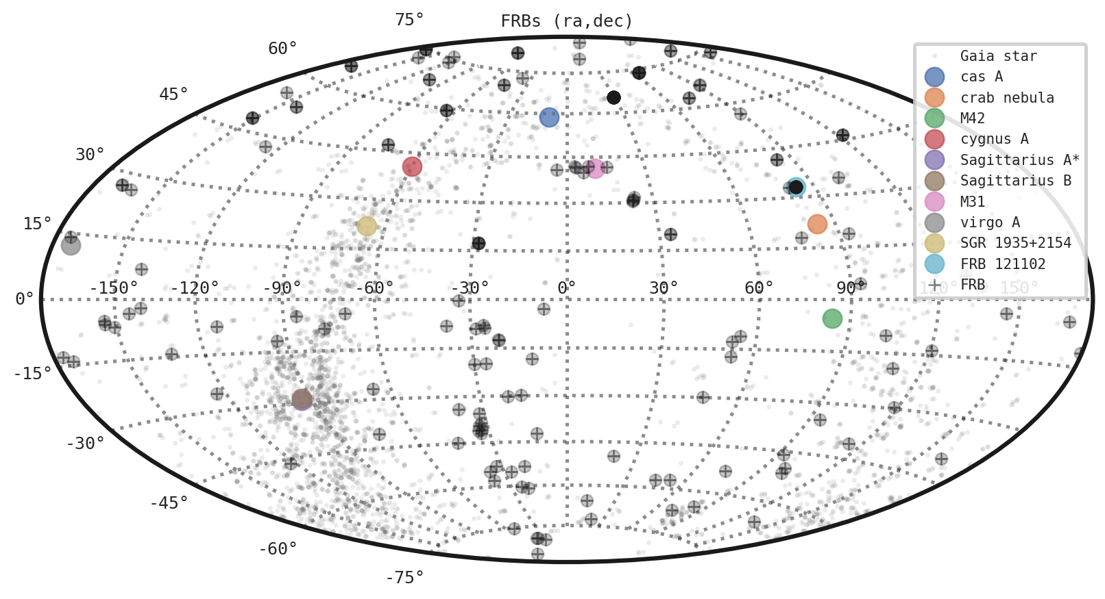

galactic coordinates

# plot galactic
      plt.figure(figsize=(11,7), dpi=180)
      plt.subplot(111, projection="hammer") # options: "mollweide", "lambert", "aitoff", "hammer"
      plt.title("FRBs (l,b)")
      plt.grid(True, linestyle='dotted')
      plt.plot(stars_l_rad, stars_b_rad,'o', markersize=2, alpha=.1, color='gray', label="Gaia star")
      for i,s in enumerate(sources):
          plt.plot(src_galactic_lon[i], src_galactic_lat[i], 'o', markersize=11, alpha=.75, label=radio_sources[i])
      plt.plot(galactic_lon, galactic_lat, '+', markersize=7, alpha=0.55, color='k', label="FRB")
      plt.plot(galactic_lon, galactic_lat, 'o', markersize=7, alpha=0.25, color='k')
      plt.legend(fontsize='small',loc='upper left');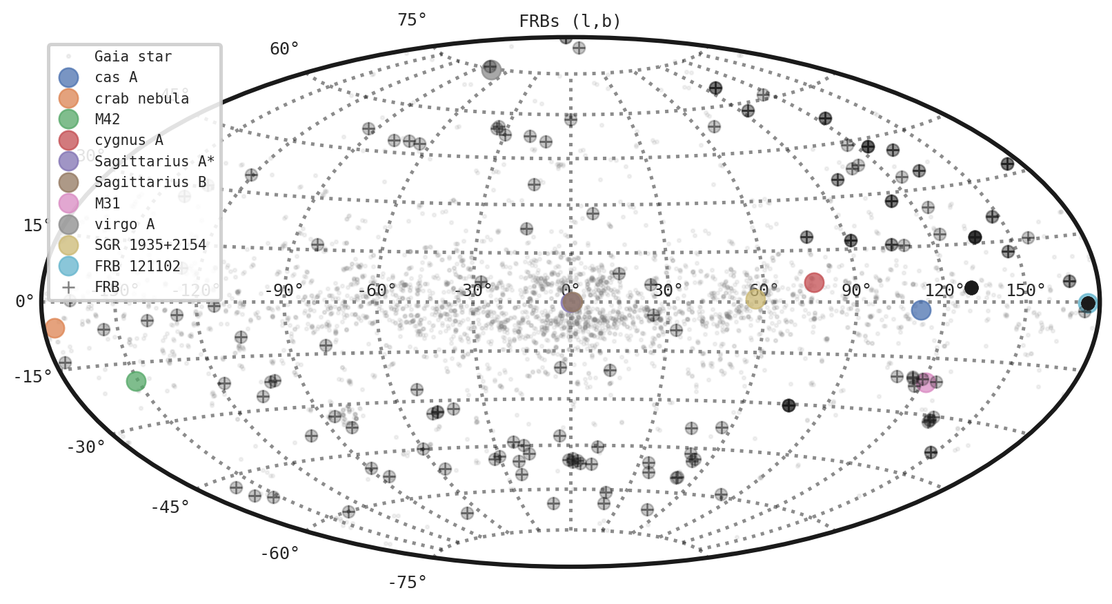

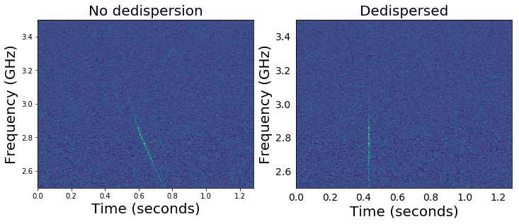
Dispersion relations, lightning, and redshift

Alfven waves, which are transverse waves on magnetic field lines, have zero dispersion. In general, dispersion relations relate the wavelength/wavenumber ( $\lambda/k$ ) to its frequency $\nu$ . The dispersion relation form

$v(\lambda) = \lambda \nu(\lambda)$

shows how the velocity of the wave is a function of wavelength/frequency. Typically, the well-known relation is $c = \lambda \nu$ for electromagnetic waves. This can result in an emission with a bandwidth getting spread out or dispersed and requires a medium for electromagnetic waves, as the example of a prism with an index of refraction yielding a dispersion relation. The other way to represent a dispersion relation more geometrically is

$\omega(k) = v(k) k$

where $k$ is the wavenumber $2\pi / \lambda$ and $\omega$ is the angular frequency $2\pi \nu$ . This allows the group and phase velocities to be more readily accessible:

$v_{phase} = \frac{\omega}{k}$ $v_g = \frac{\partial \omega}{\partial k}$

The following image shows a single FRB and is a good visualization of dispersion, i.e., phase velocity being dependent upon frequency. The image is from https://github.com/caseyjlaw/FRB121102/blob/master/demo_FRB121102.ipynb and is showing data that was used for the first localization of a FRB with the VLA [Chatterjee2017].

fast radio burst FRB121102 — FRB121102 [https://github.com/caseyjlaw/FRB121102/blob/master/demo_FRB121102.ipynb]

# FRB chirp -- terminology
	  HTML('<video width="887" height="499" controls> \
	                       <source src="videos/FRB_chirp.mp4" type="video/mp4">\
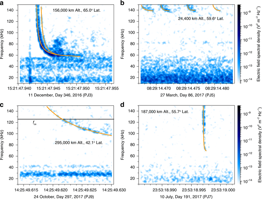
	                       </video>')

# Whistlers -- local electromagnetic observations
	  HTML('<video width="800" height="600" controls>\
	          <source src="videos/whistlers.mp4" type="video/mp4">\
	          </video>')

Lightning like examples have been shown before in the solar system and farther away [Aleksi__2014]. This is an example from Jupiter [Imai2019].

Dispersion measure $DM$ is one of the values reported for the FRBs. For pulsars this quantity is defined as the integral of free electron density over the line of sight path to the pulsar

$DM = \int_{\mathcal{P}} n_e ds$

where $n_e$ is the free electron density and $ds$ would be an infinitesimal line element for the path $\mathcal{P}$ , which should be defined by a metric for extragalactic observations. For FRBs the integral typically is written as [Zhang2020]

$\int_{\mathcal{P}} \frac{ n_e(s) }{ 1 + z(s) } ds$

where the variability of $n_e(s)$ is parameterized and cosmic expansion factored in with the redshift factor $z(s)$ .

# show dispersion measure distribution
	  plt.figure(figsize=(11,7), dpi=180)
	  bins = plt.hist(frb_catalog['dm [pc/cm^3]'].astype('float'), cumulative=False, bins=25,
	                  histtype='stepfilled', alpha=1, color='gray')
	  plt.xlabel('Dispersion Measure [pc/cm^3]')
	  plt.ylabel('# of FRBs');

There is a good write up about the lightning analog here: https://www.explainxkcd.com/wiki/index.php/2027:_Lightning_Distance

The magnetar hypothesis

# calculation
	  l_frb = (constants.c*.001*u.s).to(u.km)

A FRB was localized to a known magnetar on April 28th, 2020. Repeating FRBs are much easier to localize as they can be observed with higher resolution telescopes that are too precise for initial detection. This might bias the evidence towards repeating FRBs, which would be biased towards periodic sources like pulsars. The “width” (length in time) of any given FRB is on the order of milliseconds as the units above might indicate. This fact has been used to extrapolate a length scale by multiplying this time by the speed of light to get the result [Zhang2020]:

$\mathcal{l}_{FRB} \le c w_{FRB}$

where the length scale ends up being roughly 300 km. This is about a micro-au (!), so if this analysis is to be believed then it certainly points towards compact objects like white dwarfs, black holes, and neutron stars.

The width of FRBs appears to follow the power law behavior of scattering in cold plasma [Zhang2020]

$w \propto \nu^{-4\pm 1/2}$

Follow up observations at other wavelengths have imaged the magnetar in question [Bailes_2021].

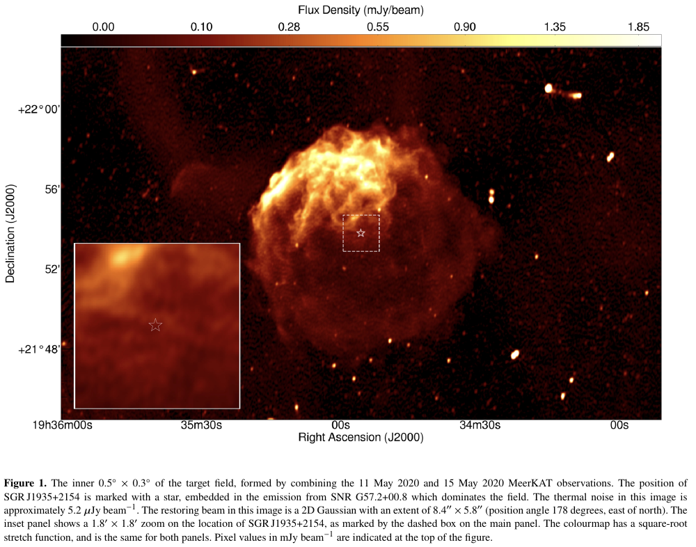
This was associated with FRB200428. This is one of ~20 known magnetars within the Milky Way.

<< Time domain astronomy and imaging techniques >> *

Cosmological questions

# make fruitbat objects to calculate redshift
	  fb_objs = []
	  for dm in frb_catalog['dm [pc/cm^3]']:
	      fb_objs.append(fruitbat.Frb(float(dm)))

# generate cosmology data
	  cosmologies = ['WMAP5', 'WMAP7', 'WMAP9', 'Planck13', 'Planck15', 'Planck18', 'EAGLE']
	  redshifts = []
	  for cosmo in cosmologies:
	      redshifts.append( np.array( [ float(fb_objs[i].calc_redshift(cosmology=cosmo)) \
	                                   for i in range(len(fb_objs)) ]) )
	  rsdf = pd.DataFrame(data=redshifts, index=cosmologies)
	  rsdfs = rsdf.stack()
	  rsdfs.name = 'redshifts'
	  df_tidy=rsdfs.reset_index()
	  # df_tidy['redshifts'] = np.log(df_tidy['redshifts'])

# plot redshift for each FRB for each cosmology
	  sns.set(context="poster", style="whitegrid",
	          rc={'grid.alpha':.5, 'grid.linestyle':'dotted', 'grid.color':'k',
	              "lines.linewidth":2.5, "axes.edgecolor":'k',
	              'legend.facecolor':'w', 'text.usetex':False, 'mathtext.fontset':'cm',
	              'legend.fontsize':'x-small', 'legend.framealpha':0.88,
	              'axes.formatter.use_mathtext':True, 'figure.dpi':180, 'font.family':'monospace',
	             "figure.facecolor":'none', 'axes.facecolor':'none'})
	  with warnings.catch_warnings():
	      warnings.simplefilter("ignore")
	      splt = sns.jointplot(data=df_tidy, x='level_1', y='redshifts', hue='level_0', kind='kde',
	                           palette=sns.color_palette('cubehelix', 7),
	                    space=0, height=11, ratio=7, s=155)
	      splt.set_axis_labels('FRB', 'z')

Can FRBs help to map the hard-to-see filimentary structure between galaxies?
Might they provide better constraints on geometry/curvature (consider pulsar accuracy)?
What about dark energy and dark matter?

References

[Zhang2020] Zhang Bing, ``The physical mechanisms of fast radio bursts’’, Nature, vol. 587, number 7832, pp. 45-53, Nov 2020. online

[Chatterjee2017] Chatterjee C. J. and et al., ``A direct localization of a fast radio burst and its host’’, Nature, vol. 541, number 7635, pp. 58-61, Jan 2017. online

[Aleksi__2014] Aleksić J., Ansoldi S., Antonelli L. A. et al., ``Black hole lightning due to particle acceleration at subhorizon scales’’, Science, vol. 346, number 6213, pp. 1080–1084, Nov 2014. online

[Imai2019] Imai Masafumi and et al., ``Evidence for low density holes in Jupiter’s ionosphere’’, Nature Communications, vol. 10, number 1, pp. 2751, Jun 2019. online

[Bailes_2021] Bailes M, Bassa C G, Bernardi G et al., ``Multi-frequency observations of SGR J1935+2154’’, Monthly Notices of the Royal Astronomical Society, vol. , number , pp. , Mar 2021. online